Introduction

There exists a large, oftentimes vocal, community of investors who strongly favor dividend-paying stocks. In fact, dividends are a core element of many Financially Independent Retire Early (FIRE) portfolios. Are dividend-paying stocks special?

Simple financial models say no. There’s nothing intrinsic about a dividend that enhances the return of the stock that paid it. A company has cash on its balance sheet. It distributes some cash to its investors in the form of a dividend. Now the investor has some cash, and the company’s cash balance has been equivalently reduced. Thus, the economic value of the company declines by the same amount. The dividend paid is associated with an offsetting capital loss. The total return attributable to a dividend is zero. Several papers have shown this to be approximately true (Campbell and Beranek, 1955; Black and Scholes, 1974; Barclay, 1987; Boyd and Jagannathan, 1994). There’s little reason to find a dividend appealing. In fact, dividends generate a tax liability and investors who receive dividends lose some control over when they realize taxes versus investors who own non-dividend paying stocks (Israel et al., 2019).

Potential counterpoint. A dividend itself might have no impact on total performance, but stocks that pay dividends might have characteristics that are associated with performance. For example, dividend payers might tend to be value stocks and defensive stocks, both of which are factors that have demonstrated positive performance. While the dividend itself is economically immaterial, the signal that it conveys might matter.

Let’s get to the bottom of this.

We split stocks in our universe into high-dividend and low-dividend groups by their median dividend yield in the previous year and study the impact of dividends on investment returns under two different settings. In the first setting, we compare the performance of the two different groups and test if the high-dividend group has historically outperformed the low-dividend group. In the second setting, we apply a dividend-based portfolio adjustment to a few long-only factor portfolios to test the hypothesis that active investors can benefit from restricting their selection of factor winners among high-dividend groups. More specifically, we penalize the target weight of low-dividend stocks in the portfolio regardless of their factor scores. If low-dividend stocks predict lower future returns in addition to the factor portfolio, we should expect stronger performance under the new construction.

Our results indicate that while the high-dividend group has indeed delivered better returns than the low-dividend group, the outperformance can be entirely explained by a set of common quant factors. After controlling for value, quality, and defensive factors, the excess return of high-dividend over low-dividend turns negative. In other words, our analysis suggests that investors who seek to achieve alpha should invest directly in a combination of these factors instead of holding high-dividend stocks.

Tilting long-only factor portfolios towards high-dividend stocks has in general a negative effect on performance. For factors that are naturally correlated with dividend yield, the additional adjustment has little impact on gross performance but results in lower net returns due to the tax burden of dividend incomes (in taxable accounts). On the other hand, the filter is too restrictive for the momentum factor, which is essentially uncorrelated with the dividend yield, causing a large reduction in implementation efficiency and hence investment returns.

All things considered, the dividend yield is just a poor proxy for a value, quality, and defensive-based multi-factor strategy. Our analysis demonstrates that active investors should not constrain their portfolios based on dividend yields.

Literature Review

Our paper builds upon the literature on the relationship between dividend yield and stock returns. The theoretical model in Miller and Modigliani (1961) suggests that if dividend policy does not affect the corporation’s investment decisions, it should not have any impact on the value of its shares at all. Subsequent empirical studies test this hypothesis directly and find mixed results (Black and Scholes, 1974; Litzenberger and Ramaswamy, 1979; Miller and Scholes, 1982). As Black and Scholes (1974) point out, establishing a causal relationship is challenging because it is very difficult to control for variables other than dividend policy.

Nevertheless, there is strong evidence that dividend yield is positively correlated with the cross-section of expected stock return and cannot be explained solely by tax effects (Fama and French, 1988, 1993; Christie, 1990; Naranjo et al., 1998). Sialm (2009) sorts stocks into dividend portfolios and reports that stocks with high-dividend yields have significantly higher average abnormal returns than stocks without dividends, even after various factor adjustments. Hameed et al. (2022) provide strong international evidence of dividend-payers outperforming non-payers in 44 countries. However, Swedroe (2023) shows that the dividend premium in the US stock market has negative alphas against the Fama-French five-factor model (Fama and French, 2015).

Our paper also relates to studies on after-tax returns of active portfolios. Jeffrey and Arnott (1993, 2018) find that most actively managed funds cannot outperform the S&P 500 index funds on an after-tax basis. In their sample, mutual funds have an average annual tax burden of 1.1% due to capital gains and dividends. Bergstresser and Pontiff (2013) use the federal tax codes from 1926 through 2007 to construct the after-tax returns on a set of factor portfolios and find that even though the size and value factors still generate positive after-tax returns, the magnitudes are much smaller than those suggested in the tax-exempt version by Fama and French (1993). Using a shorter period from 1995 through 2018, Goldberg et al. (2018) show that the tax burdens of long-only portfolios with factor tilts can be mitigated through tax loss harvesting. Israel and Moskowitz (2012) compare the after-tax returns of size, value, growth, and momentum strategies. They find that the tax exposure of the value strategy primarily comes from dividends, while momentum’s is mostly driven by realized capital gains.

Conceptually, our analysis on the interaction between active portfolio returns and dividend yield complements Israel et al. (2019). They find that even though dividend stocks are tax inefficient, investors should still keep them in their portfolios because avoiding them materially lowers the factor alpha. The reduction is particularly pronounced for factors with naturally high dividend yields. Our study addresses the opposite question: given dividend stocks’ outperformance over non-payers, could investors benefit from building active portfolios entirely with high-dividend stocks, both before and after tax? The two papers also differ in methodology. Israel et al. (2019) introduce a dividend aversion parameter to a complex optimization objective function and study the output under various aversion inputs. We employ a direct sorting and dividend-filtering method for active portfolio construction, which gives practitioners better intuition over the trade-offs between factor exposures and dividends, as well as more control over the implementation process.

Data and Methods

Our analysis covers the period beginning January 1964 and ending December 2021. Stock prices, returns, and dividends are from the Center for Research in Security Prices (CRSP). Risk-free rates are from the Kenneth French Data Library. Our regression analysis includes several factors with sources specified as follows. The factor returns of the 5-Factor Fama-French model, which include the market (MKT), size factor (SMB), value factor (HML), profitability factor (RMW), and investment (CMA), come from the Kenneth French Data Library. We augment the model with the momentum factor (UMD) and a defensive factor (BAB), which both are downloaded from the AQR Data Library.

Our equity universe consists of the top 1,500 common stocks, sorted by market capitalization as of the last trading day of the prior year. We seek to better understand the properties of portfolios that give preferential treatment to high dividend-paying stocks. To do so, we stratify our universe into a high-dividend group and a low-dividend group and compare the properties of these stocks to each other and also to the full universe.

A natural stratification method would split stocks as dividend-payers and non-payers. However, as documented in Fama and French (2002) and Michaely and Moin (2022), the fraction of companies that issue dividends varies greatly over time. Fewer firms paid dividends from the 1970s to the 2000s, but the trend has reverted since then. We observe the same pattern in our universe: more than 80% of the stocks paid dividends in the 1970s and the fraction declined constantly to about half in the 2000s and increased back to 60% in recent years.

To keep the two groups more balanced in their number of stocks, we divide our universe into two halves based on their prior year’s dividend yields. Stocks above the median yield fall into the high-dividend group and the bottom half are in the low-dividend group.¹ In doing so, the diversification properties of the two sub-groups are similar by design.

Historical Performance of the Dividend Stocks

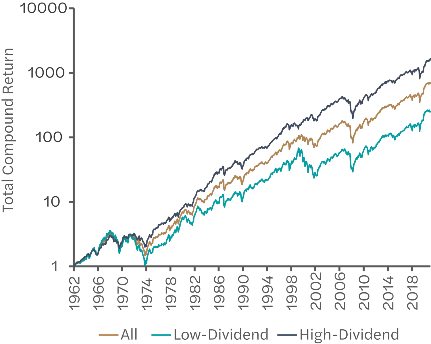
We form three equal-weight portfolios using stocks in the high-dividend group, low-dividend group, and the entire universe respectively. Exhibit 1 plots the cumulative performance of the three portfolios. The high-dividend portfolio clearly dominates the other two groups both in return and risk. It realized a 13.8% average annual return with 15.6% volatility. In comparison, the low-dividend portfolio realized lower returns (11.8%) with much higher volatility (21.9%). The higher return and lower volatility result in a material 3.6% difference in compound annual growth rate (CAGR)!

The high-dividend portfolio also has smaller drawdowns during market corrections. After the dot-com bubble, the low-dividend portfolio tanked 62.8% while the high-dividend portfolio dropped merely 19%. Interestingly, the peak-to-trough drawdowns of the two portfolios are much closer during the Global Financial Crisis. The high-dividend and low-dividend portfolios lost 57% and 54.2% respectively.

Exhibit 1: Cumulative Performance of High-Dividend and Low-Dividend Portfolios

This exhibit plots the cumulative performance of stocks in three groups using historical data from 1963 to 2021. All represents the full universe, and Low-Dividend and High-Dividend represent the bottom- and top-half of dividend-yielding stocks respectively. Each portfolio is capitalization weighted. Our investment universe is the top 1500 stocks by market capitalization. Each year, stocks are sorted into the high-dividend and low-dividend groups by the median dividend yield in the previous year. The historical data of stocks comes from CRSP and the risk-free rate is from Kenneth R. French Data Library.

Source: NDVR, Center for Research in Securities Prices, French Data Library

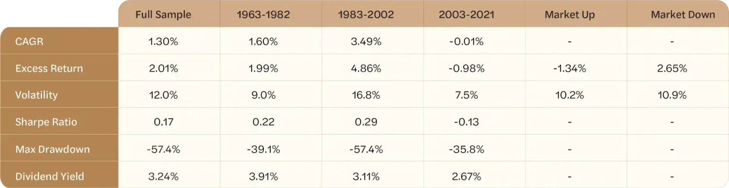
Next, we construct a long-short portfolio that holds the high-dividend portfolio and shorts the low-dividend portfolio. We refer to the portfolio’s return as the Dividend Spread. Exhibit 2 reports the performance of the Dividend Spread across the full sample as well as three sub-periods. Despite the high-dividend stocks’ outperformance in the full sample, investment in this long-short portfolio lost close to 1% per year between 2003 and 2021. Most of the positive returns came from the middle twenty-year period from 1983 to 2002 with the highest annualized return of 4.86%. This period also has the largest drawdown of 57.4%, which occurred during the dot-com bubble when growth tech companies rallied.

Another interesting pattern is that the dividend gap, which measures the difference in dividend yield between the two portfolios, decreases over time from 3.91% in the early sample period to 2.67% in the last period. Since total return is the sum of price return and dividend yield, we can infer that high-dividend stocks on average have 1.23% lower price returns per year than low-dividend stocks over the full sample period and 3.65% lower in the last sub-period.

Exhibit 2: Performance of the Dividend Spread

This table reports the sub-period performance metrics of the Dividend Spread using historical data from 1963 to 2021. The Dividend Spread is defined as the difference between the equal-weight high-dividend portfolios and the equal-weight low-dividend portfolios. Our investment universe is the top 1500 stocks by market capitalization. Each year, stocks are sorted into the high-dividend and low-dividend groups by the median dividend yield in the previous year. The historical data of stocks comes from CRSP and the risk-free rate is from Kenneth R. French Data Library.

Source: NDVR, Center for Research in Securities Prices, French Data Library

Can Existing Factors Explain the Dividend Spread?

What explains the performance of the Dividend Spread? Does it have alpha?

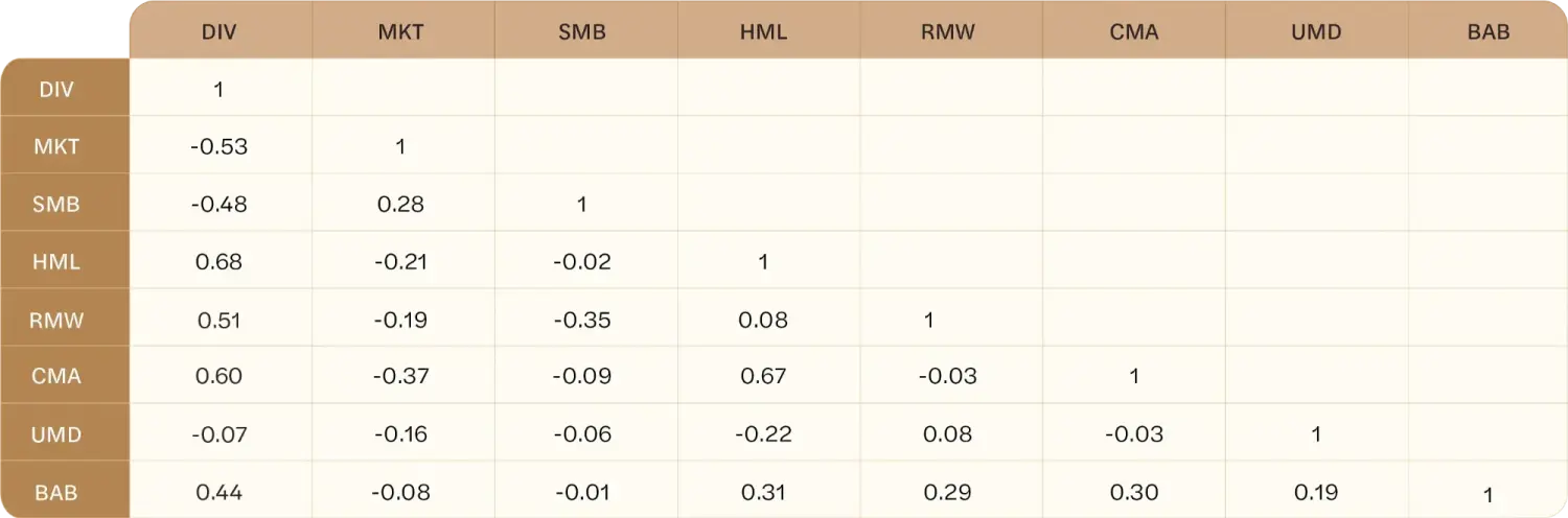
To investigate the source of its outperformance, we estimate the Dividend Spread’s exposure to a set of well-known factors used by researchers and practitioners. Exhibit 3 reports the correlation matrix among the dividend spread and the six factors. The dividend spread has a negative correlation with MKT (-0.53) and SMB (-0.48), and a positive correlation with BAB (0.44), suggesting the high-dividend portfolio contains larger stocks with smaller market betas compared to those in the low-dividend portfolio. The spread is also positively correlated to HML (0.68), RMW (0.51) and CMA (0.60). It confirms Swedroe’s (2023) findings and also the intuition that stocks without dividends tend to be growth stocks with lower profitability and more aggressive investment. There is a small negative correlation between the spread and the momentum factor.

Exhibit 3: Correlation Matrix of Dividend Spread and Risk Factors

This table reports the correlation among Dividend Spread and uses historical data from 1963 to 2021. The Dividend Spread is defined as the difference between the equal-weight high-dividend portfolios and the equal-weight low-dividend portfolios. Our investment universe is the top 1500 stocks by market capitalization. Each year, stocks are sorted into the high-dividend and low-dividend groups by the median dividend yield in the previous year. The historical data of stocks comes from CRSP. The risk-free rate, MKT, SMB, HML, RMW, CMA and UMD return series are from Kenneth R. French Data Library. BAB return series comes from the AQR Data Library.

Source: NDVR, Center for Research in Securities Prices, French Data Library, AQR Data Library

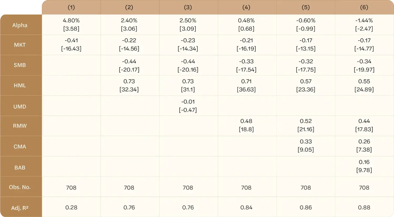
We extend the correlation analysis and regress the Dividend Spread’s return on these factors’ returns to test whether the long-short portfolio has any excess return beyond the existing factor premiums. We have seen that despite the headwinds from a negative market exposure, the spread has generated an average positive return of 1.3% per year. Regression 1 in Exhibit 4 shows that adjusting for the portfolio’s negative market beta of -0.41, the dividend spread has an even more impressive CAPM alpha of 4.8%.

However, the excess return drops by half to 2.4% after controlling for size and value factors. The Dividend Spread’s loading on the value factor contributes to more than 2% of its CAPM alpha. Furthermore, the adjusted R-squared value also jumps from 28% to 76%. More than three-fourths of the time-series variation in the dividend spread can be explained by the Fama-French three factors. Adding the momentum factor has no impact on the regression model: its coefficient is neither economically nor statistically significant. Hence, we do not include the momentum factor in subsequent regressions.

However, the excess return drops further to 0.48% and becomes statistically insignificant after adding the profitability factor. In the full model, after controlling for Fama and French’s (2015) five-factor model plus BAB, the regression’s adjusted R-squared value increases to 88% and the Dividend Spread has a statistically significant negative alpha of -1.44% per year. Consistent with Swedroe (2023)’s results, the dividend spread has negative loadings on MKT and SMB, and positive loadings on HML, RMW, CMW and BAB.

All regression coefficients are highly significant. The regression results show that the Dividend Spread’s outperformance is [more than] completely explained by a set of well-known factors. In fact, investors could have avoided incurring the negative excess returns if they had held a combination of these factors rather than investing in the dividend-based long-short portfolio.

Exhibit 4: Regressions of Dividend Spread on Risk Factors

This table reports the coefficient estimates and annualized alpha of regressing the Dividend Spread on a set of common factors using historical data from 1963 to 2021. The Dividend Spread is defined as the difference between the equal-weight high-dividend portfolios and the equal-weight low-dividend portfolios. Our investment universe is the top 1500 stocks by market capitalization. Each year, stocks are sorted into the high-dividend and low-dividend groups by the median dividend yield in the previous year. The historical data of stocks comes from CRSP. The risk-free rate, MKT, SMB, HML, RMW, CMA and UMD return series are from Kenneth R. French Data Library. BAB return series comes from the AQR Data Library.

Source: NDVR, Center for Research in Securities Prices, French Data Library, AQR Data Library

Dividend Stocks and Active Factors

We’ve gained some insight by looking at a long-short portfolio constructed on dividend yields. These insights do not necessarily translate to long-only portfolios when shorting is impermissible. We now turn our attention to whether long-only investors would have benefited by favoring high-dividend stocks. We focus on active portfolios in our analysis because those investors who favor high dividend-paying stocks have a revealed preference for active management.

Our analysis is straightforward. We first consider an active long-only portfolio constructed over the full universe of stocks. Next, we consider a similarly constructed long-only portfolio after filtering the universe to only include high-dividend stocks. We horserace these two portfolios against each other.

If dividend-paying stocks have favorable return profiles to non-payers, one might expect better performance after removing low-dividend stocks from portfolios. On the other hand, constructing factor portfolios with a restricted universe has a negative impact on the overall factor exposure and alphas (Chen and Israelov, 2023). Hence it is unclear what the net effect is.

We run our horserace on portfolios constructed on three types of factors: momentum, value, and safety/defensive, each of which are all well-established among academic researchers and practitioners.² Our momentum and value signals follow the traditional definition: sorting stocks based on T-12 to T-1 month returns and book-to-market ratios respectively (Fama and French, 1993; Carhart, 1997). To construct the safety factor, we use stocks’ “slope-winsorized” market betas, estimated using daily returns in the previous year (Frazzini and Pedersen, 2014; Welch, 2019). In addition to the individual factors, we also consider a composite factor using an equal-weighted average of ranks derived from the three sets of factor scores.

Equal-weight Portfolios

First, we consider equal-weight factor portfolios as the benchmark, which can inform us of the gross signal returns, but are usually not implementable due to their high turnovers. For each factor we consider, we equally weight the top 300 stocks ranked by the factor scores. This represents the top quintile of stocks within the full universe and the top two quintiles within the high-dividend universe.

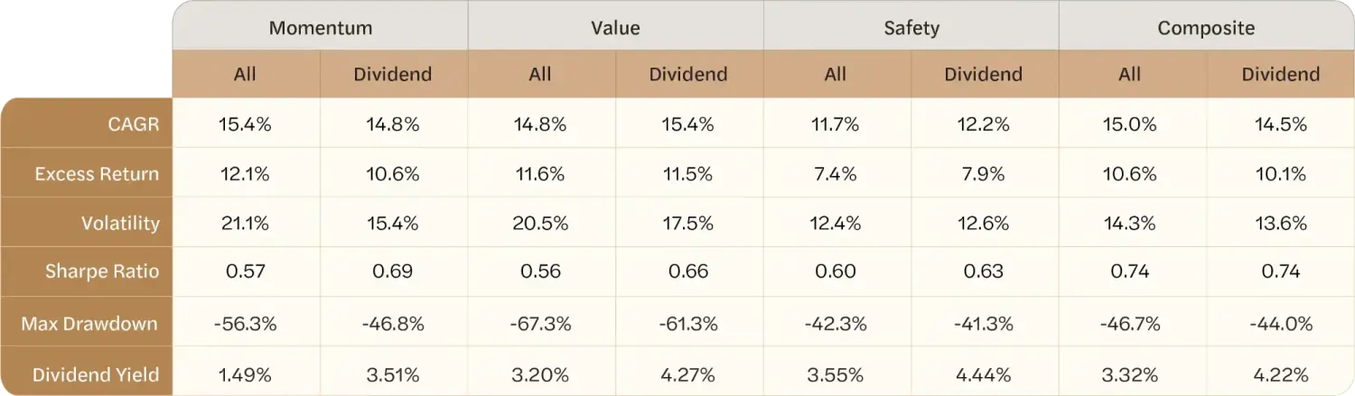
Exhibit 5 summarizes the performance metrics of the four factor portfolios constructed under the two construction methods. Consistent with the findings in Chen and Israelov (2023), the momentum portfolio is most impacted by the universe restriction. Its annual excess return drops from 12.1% to 10.6% after we filter the investible universe by dividends. The impact on other factors is much smaller. Safety gained 50bps returns per year under the high-dividend universe while value and the composite factor lost 10bps and 50bps, respectively.

As expected, the portfolios are also different in their dividend yields, but these higher yields do not necessarily translate to higher returns. Take momentum for example: despite having a 2% higher dividend yield, the high-dividend momentum portfolio had a 1.5% lower total return. This implies that its price return was 3.5% lower than that of the full universe momentum portfolio. Given dividends and price returns have different tax implications, the difference in dividend yields can potentially impact the after-tax net returns. We will address this issue in later sections.

Exhibit 5: Equal-weight Portfolio Performance Using Full and High-Dividend Universe

This table reports the performance of equal-weight factor portfolios using historical data from 1963 to 2021. Our investment universe is the top 1500 stocks by market capitalization. Each year, stocks are sorted into the high-dividend and low-dividend groups by the median dividend yield in the previous year. The all-stocks portfolios are constructed using the top 300 winners among the entire universe, whereas the dividend portfolios are constructed using the top 300 winners in the high-dividend group. The signals we use to construct the value portfolio are from Chen and Zimmermann (2022). The historical data of stocks come from CRSP. The risk-free rates are from Kenneth R. French Data Library.

Source: NDVR, Center for Research in Securities Prices, French Data Library, AQR Data Library

The high-dividend factor portfolios have in general realized higher Sharpe Ratios than their full universe counterparts. Except for safety portfolios, this improvement is mostly driven by lower volatility. On the surface, it seems contradictory to the findings in Chen and Israelov (2023) that factor portfolios constructed with a restricted universe in expectation should underperform the unconstraint portfolio (Asness, 2017). However, the results in Chen and Israelov (2023) are based on portfolios with random exclusions since the goal of the exercise is to quantify the average impact of stock exclusions.

In this paper, we are interested in one particular set of stocks with a carefully chosen characteristic: high-dividend stocks. Given we have shown that these stocks have high exposures to well-known factors such as value, quality, and safety, increasing weights to high-dividend stocks is similar to loading on these factors. Blitz and Vidojevic (2018) show that removing stocks unfavored by other factors can improve the performance of generic single-factor portfolios, which is consistent with our findings here.

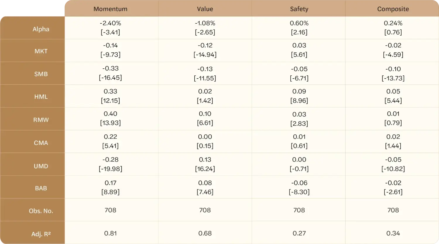
To better understand the difference in factor exposures, we regress the spread between the high-dividend active portfolios and the full-universe active portfolios on the same set of common factors. Exhibit 6 reports the regression results. Except for the safety factor, restricting the factor portfolio to high-dividend stocks does not yield statistically significant excess returns once we control for the underlying factors. On the contrary, the momentum spread portfolio loses 2.4% alpha and the value spread portfolio loses 1.08%.

The factor exposures of the Dividend Spread in active portfolios are similar to what we have seen in passive portfolios. In general, the Dividend Spread loads negatively on the market and size factor as dividend stocks tend to be larger stocks with lower market beta. It also increases the factor exposures to HML, RMW and BAB. Interestingly, while the dividend spread in passive portfolios is essentially uncorrelated with UMD, restricting the universe to high-dividend stocks has a stark negative impact on UMD. This is because on average the high-dividend momentum portfolio is unable to hold half of the top 300 stocks it would hold under the full universe, which substantially reduces the average factor rank in the portfolio. On the other hand, the high-dividend universe is much less restrictive in the other three factors since they are naturally biased towards stocks that pay dividends.

Exhibit 6: Regressions of the Active Portfolio Dividend Spread on Risk Factors

This table reports the coefficient estimates and annualized alpha of regressing the active portfolio dividend spread on a set of common factors using historical data from 1963 to 2021. Our investment universe is the top 1500 stocks by market capitalization. Each year, stocks are sorted into the high-dividend and low-dividend groups by the median dividend yield in the previous year. The dividend spread is defined as the difference between the factor portfolio constructed using the high-dividend group and the same factor portfolio using the entire universe. The signals we use to construct the value portfolio are from Chen and Zimmermann (2022). The historical data of stocks come from CRSP. The risk-free rate, MKT, SMB, HML, RMW, CMA and UMD return series are from Kenneth R. French Data Library. BAB return series comes from the AQR Data Library.

Source: NDVR, Center for Research in Securities Prices, French Data Library, AQR Data Library, Chen and Zimmermann (2022)

A Practical Implementation of Factor Portfolios

While these equal-weight portfolios can inform us on the strength of the signals in generating excess returns, investors who attempt to implement them in practice will face many obstacles. First, maintaining equal weights in every stock will require frequent and large rebalances as stock positions drift away from the equal-weight targets from price movement.

Moreover, since these adjustment trades are contrarian in nature (i.e., cutting weights back from stocks that have performed well in recent periods), it is extremely tax inefficient. Finally, equal-weight portfolios naturally have positive loadings on the size factor since they tilt more active weights toward small stocks. Trading in and out of those positions also raises liquidity concerns (Swade et al., 2023). Hence, we propose a practical rebalancing algorithm that adds factor tilts to a benchmark portfolio.

We start from a market-cap-weighted portfolio and reduce the weight of factor losers in the portfolio. The excess active weight is then re-assigned to factor winners. Following the recommendation of Israelov and Lu (2023), we impose a variety of limits to control turnover and the overall active risk. For simplicity, we impose the same level of active weight allowance for both factor winners and losers. The underweight limit does not bind for the majority of the stocks with low benchmark weight, but restricts the portfolio from liquidating large benchmark names in their entirety should they become factor losers. On the other hand, the overweight limit always binds unless the portfolio is running out of available capital for investment.

Even though we have active weight constraints to ensure the initial position size of each stock is close to its benchmark weights, over time their sizes will naturally diverge further. If a factor winner outperforms its peers, its active weight will also grow proportionally. What happens when stocks drift too far from their benchmark weights? It is undesirable from a diversification perspective to have concentrated large active weights in a few stocks. We define a trigger-based rule that rebalances the stock back to target when its active weight crosses the upper or lower threshold.

Unfortunately, the impacted positions are likely those with the strongest investment gains and are thereby likely to create taxable gains. To reduce the need for frequent adjustment, we set a wider threshold relative to the active weight allowance for factor winners. Finally, we impose a minimum transaction size to avoid small nuisance transactions that may not justify any fixed trading costs.

Once we have set the parameters and rules, the rebalancing algorithm can be broken down into the following steps:

Algorithm for determining sales

1. Reduce overweights: Identify individual stocks that have positive active weight beyond the defined active weight constraint and sell to the benchmark weight.
2. Sell factor losers: Identify stocks in the portfolio that have migrated to the bottom of the rank by factor scores and sell to the maximum allowed underweight without violating the short-sale constraint. Round up transactions to the minimum transaction size and filter out any trades that would result in an active weight constraint violation.

Algorithm for determining buys

1. Compute cash available for purchases, which includes dividends received, as well as cash resulting from liquidations from the above-specified sales.
2. Reduce underweights: Identify and rank individual stocks that have negative active weight beyond the defined active weight constraint. Use the available cash balance to buy names up to the maximum of their perspective benchmark target.
3. Buy factor winners: Rank stocks by factor scores and purchase shares to the individual-name active weight constraint. Round up transactions to the minimum transaction size and filter out any trades that would result in an active weight constraint violation.

Active Portfolio Factor Loadings

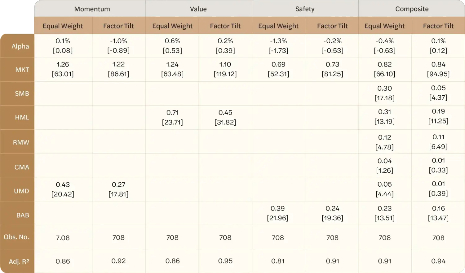
Before looking at the performance metrics, it is useful to examine how effective our proposed rebalance algorithm is at tilting the passive portfolio toward the desired factor. We regress the portfolio return on the market and the underlying factor (e.g., regressing momentum-tilted portfolio on MKT and UMD) and compare the results against the same regression with the equal-weight factor portfolios. Using the equal-weight portfolios as the factor benchmark, we can gauge how much factor exposure our algorithm achieves. Exhibit 7 summarizes the regression coefficients.

All else equal, we should expect our factor-tilted portfolios to have lower factor exposures than the equal-weight portfolios given we have a tighter constraint on the active weight allowance for factors winners. Moreover, we do not always sell non-winners and rebalance to the top-ranked stocks each month to reduce portfolio turnover. Hence the average factor rank of stocks in the portfolio should also be lower. Finally, the active underweight constraint prevents the portfolio from shunning large stocks completely even when they are not factor winners. Their presence should reduce the loading on SMB compared to the equal-weight portfolios.

The regression coefficients in Exhibit 7 show that the single-factor factor-tilted portfolios lose about 40% factor exposures relative to their equal-weight counterparts. The results for the composite portfolio are mixed because the overall effects depend on the interaction in underlying factor signals. Even though the composite signal is constructed as the equal-weight average of the three individual factors, its factor loadings indicate that the value factor and safety factor dominate the momentum factor.

Relative to the single-factor portfolios, the equal-weight composite portfolio retains 46% and 64% of the factor loadings on HML and BAB respectively. In comparison, its factor loadings on UMD drop from 0.43 in the single-factor momentum portfolio to 0.05 in the composite portfolio. It drops even further to 0.01 and becomes statistically insignificant in the factor-tilted portfolio.

Exhibit 7: Regressions of the Equal-weight and Factor-tilted Portfolios on Risk Factors

This table reports the coefficient estimates and annualized alpha of regressing the active portfolios on a set of common factors using historical data from 1963 to 2021. Our investment universe is the top 1500 stocks by market capitalization. Equal-weight factor portfolios consist of the top 300 factor winners across the entire universe. Factor-tilted portfolios are constructed following the steps under section A Practical Implementation of Factor Portfolios. The signals we use to construct the value portfolio are from Chen and Zimmermann (2022). The historical data of stocks come from CRSP. The risk-free rate, MKT, SMB, HML, RMW, CMA and UMD return series are from Kenneth R. French Data Library. BAB return series comes from the AQR Data Library.

Source: NDVR, Center for Research in Securities Prices, French Data Library, AQR Data Library, Chen and Zimmermann (2022)

Performance of Factor-Tilted Portfolios

To investigate the impact of favoring dividend-paying stocks in factor-tilted portfolios, we construct a high-dividend version of the factor portfolio by modifying the definition of a factor loser in the algorithm. In addition to penalizing stocks ranked poorly by the factor score, we also apply a negative active weight (underweight) to stocks in the low-dividend group. If the stock’s benchmark is below the underweight limit, it means we will sell/not hold the stock; if it is a large name, we will still hold it for active risk management, but at a level below its market-cap weight. The process is essentially equivalent to the construction of equal-weight portfolios under restriction: when the portfolio encounters a factor winner from the low-dividend group, instead of assigning a positive active weight, it skips the stock and assigns the active weight to the next-in-line that is from the high-dividend group.

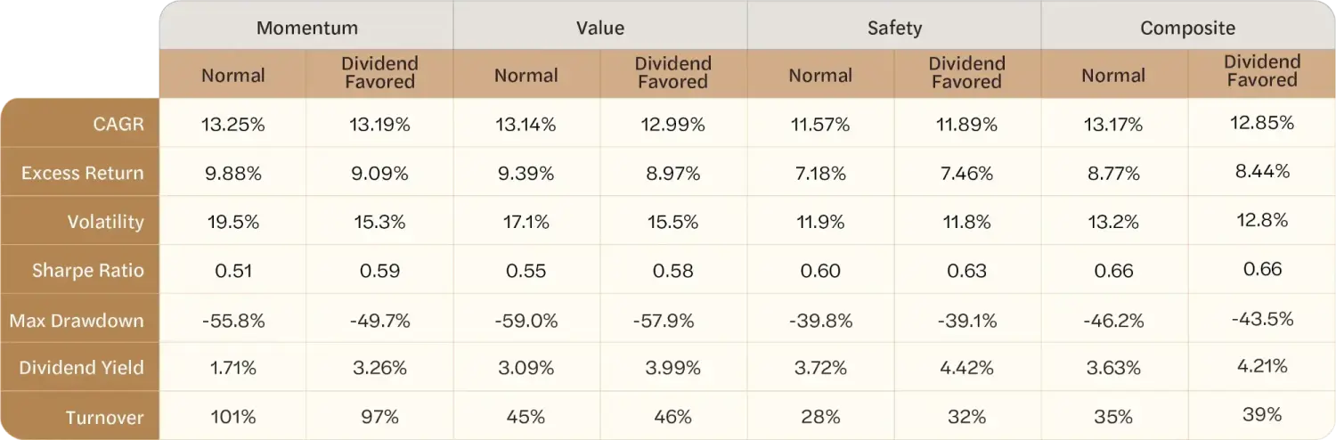
Exhibit 8 reports the gross performance of the factor-tilted portfolios under the normal rebalance algorithm and dividend-favored algorithm. The difference in the two portfolios closely matches what we saw under the equal-weight portfolio analysis, which is not surprising given our factor-tilted portfolios have the same pattern of factor exposures as their equal-weight counterparts.

Overall adding the dividend restriction has less effect on the safety and composite portfolio because they are already heavily biased toward dividend-paying stocks. The safety portfolio gains 28bps return per year while the composite portfolio loses 33bps. The momentum portfolio has the largest loss in average return at -79bps per year. At the same time, avoiding high-beta stocks through the dividend filter also benefits the most in terms of the Sharpe Ratio from the reduction in volatility.

Exhibit 8: Gross Returns of Factor-tilted Portfolios under Normal and Dividend-Favored Construction

This table reports the gross performance of long-only factor-tilted portfolios using historical data from 1963 to 2021. Our investment universe is the top 1500 stocks by market capitalization. Each year, stocks are sorted into the high-dividend and low-dividend groups by the median dividend yield in the previous year. The normal portfolios are constructed following the steps under section A Practical Implementation of Factor Portfolios, whereas the dividend portfolios are constructed in the same way, but with an underweight penalty to stocks in the low-dividend group. The signals we use to construct the value portfolio are from Chen and Zimmermann (2022). The historical data of stocks come from CRSP. The risk-free rates are from Kenneth R. French Data Library.

Source: NDVR, Center for Research in Securities Prices, French Data Library, AQR Data Library, Chen and Zimmermann (2022)

While the dividend-favored construction has improved the strategies’ Sharpe ratios, it comes at the expense of higher dividend yields and slightly more turnover. Both are undesirable for taxable investors since dividend income and realized capital gains are taxed when received. Let’s again consider the momentum portfolios as an example. The dividend-favored portfolio has a dividend yield of 3.26%, which is 1.6 percentage points higher than that of the unconstrained portfolio. Even if all dividends are qualified dividends that are taxed at a 23.8% federal tax rate, the high-dividend portfolio still loses 38bps a year.³ Since some states do not tax dividends, we do not calculate the losses due to state-level tax. Hence our estimated tax loss is on the conservative side for most investors who do not reside in a handful of dividend-tax-free States.

Following Goldberg et al. (2019), we assume an equal transaction cost of 6bps for both buy and sell for our investible universe of the largest 1,500 stocks by market cap (Frazzini et al., 2018). In addition, we also track the cumulative realized capital gains/losses and apply the appropriate short-term and long-term capital gain taxes when applicable. At the end of the investment period, we consider two terminal scenarios: without and with liquidation tax. The former assumes that the portfolio is inherited with a step-up in basis or donated tax-free. The latter assumes the entire portfolio is liquidated and the investor pays a lump-sum tax on any realized capital gains.

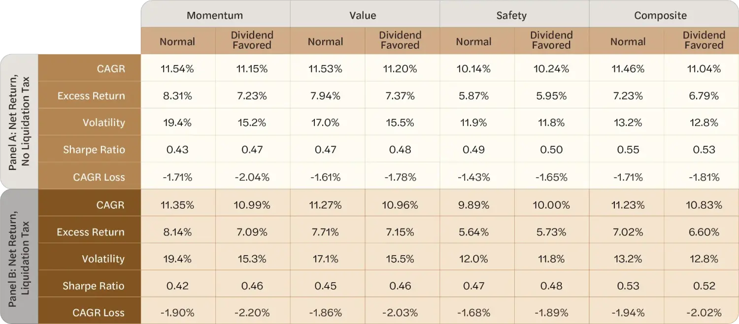
Exhibit 9 Panel A reports the net returns without liquidation tax. Once we take the tax effect into account, the dividend-favored portfolios are even less desirable in terms of CAGR. Their net CAGRs are 57bps (value) and 108bps (momentum) lower than those under the normal implementation. The last row in Panel A shows by how much gross CAGRs are lower due to taxes on dividends and realized capital gains, which are always higher under dividend-favored implementation. Interestingly, despite momentum’s reputation as a tax-inefficient strategy due to its high turnover, it has the same loss in CAGR (-1.71%) as the composite portfolios with almost three times its turnover. This is because momentum has a lower dividend yield than those value-based or defensive factors, which potentially gives it more room for tax optimization (Ross et al., 2018).

Even though the estate/donation scenario is probably more realistic given our long investment period of 59 years, one could argue that the analysis gives non-dividend-payers an advantage since they might have more unrealized capital gains that are never taxed. Hence, we report in Panel B the net returns if the investor must dissolve the portfolio and pay taxes on any embedded capital gains at the horizon end. As expected, it has a slightly bigger impact on the portfolios under the normal rebalance, which have greater cumulative price returns. However, the difference is too small to have any meaningful impact over the long horizon. For example, the normal composite portfolio loses 23bps in CAGR due to liquidation tax and its dividend-favored counterpart loses 21bps. This 2bps difference is negligible compared to their 50bps difference in pre-liquidation tax CAGR.

Exhibit 9: Net Returns of Factor-tilted Portfolios under Normal and Dividend-Favored Construction

This table reports the after-tax net performance of long-only factor-tilted momentum, value, safety, and the composite portfolios using historical data from 1963 to 2021. Our investment universe is the top 1500 stocks by market capitalization. Each year, stocks are sorted into the high-dividend and low-dividend groups by the median dividend yield in the previous year. The normal portfolios are constructed following the steps under section A Practical Implementation of Factor Portfolios, whereas the dividend portfolios are constructed in the same way, but with an underweight penalty to stocks in the low-dividend group. We assume both the long-term capital gains and dividends are taxed at 23.8% and the short-term gains are taxed at 40.8%. The transaction cost is assumed to be 6bps. The signals we use to construct the value portfolio are from Chen and Zimmermann (2022). The historical data of stocks come from CRSP. The risk-free rates are from Kenneth R. French Data Library.

Source: NDVR, Center for Research in Securities Prices, French Data Library, AQR Data Library, Chen and Zimmermann (2022)

Sub-period Performance of the Composite Portfolio

Finally, we break the composite factor portfolio into the same three sub-periods as in Exhibit 2 to test whether the variation in the Dividend Spread changes our results on dividend-favored portfolios. Given our rebalance algorithm allows the portfolio to keep previous factor winners until they become factor losers (bottom quintile), the actual positions in the portfolio are highly time-dependent. Hence, instead of splitting the long-run return series, we construct a new portfolio at the beginning of each sub-period and rebalance it until the end.

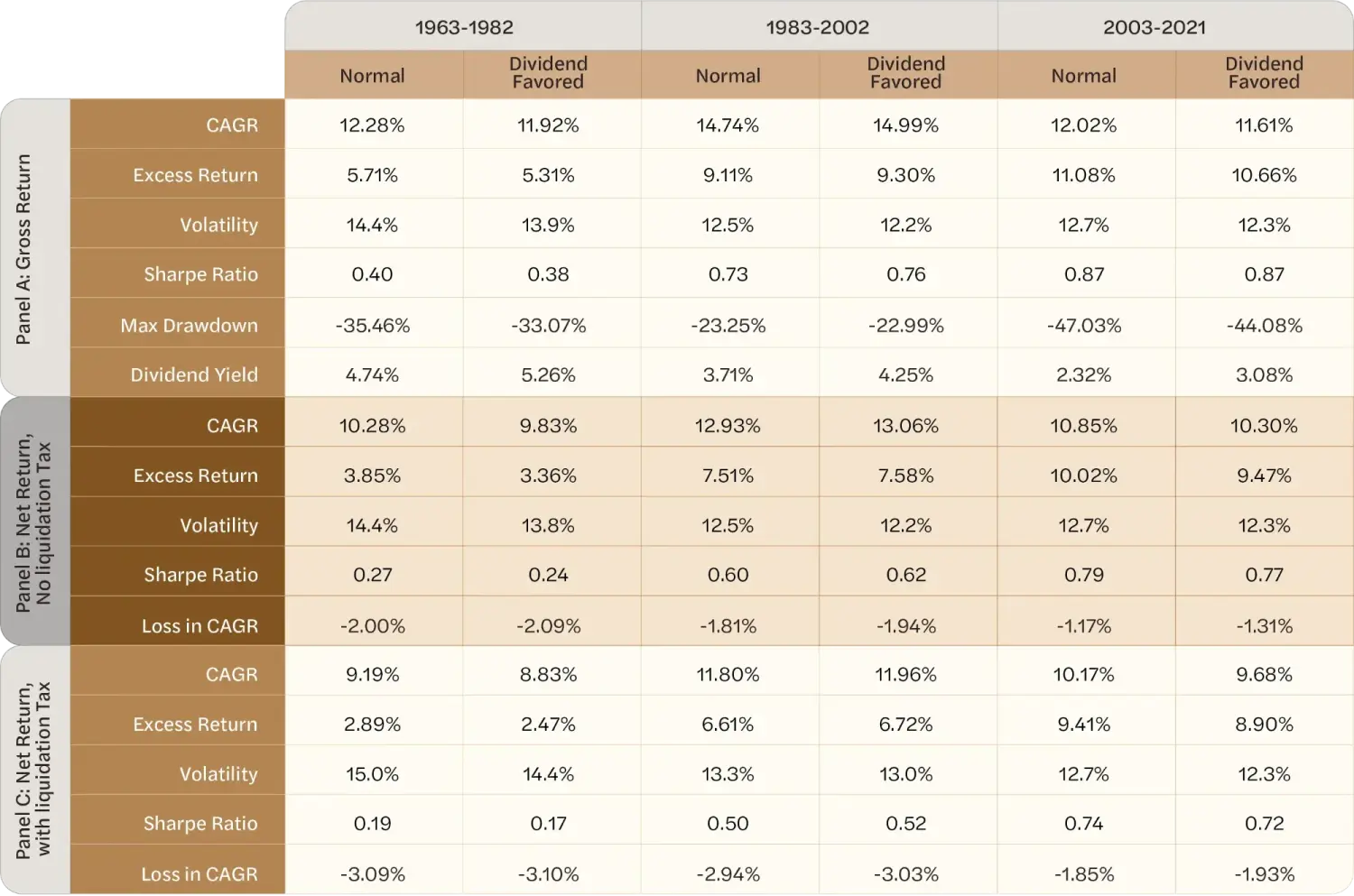
Exhibit 10 reports the gross and net performance metrics of these portfolios. Similar to what we have seen in Exhibit 2, there is a decrease in dividend yield over time from an average of 4.74% between 1963 and 1982 to 2.32% in the last sub-sample. As a result, the loss in CAGR due to taxes also trends down from -2% to -1.17% under the estate/donation scenario or from -3.09% to -1.85% with a liquidation tax.

The Dividend Spread had the best historical performance over the 1983-2002 period, which is also reflected in the dividend-favored factor portfolio. However, even under the best scenario, the dividend-favored composite factor portfolio barely outperformed the full-universe version. Its 25bps premium in gross CAGR drops to 16bps after adjusting for taxes. In the other two sub-samples, portfolios under normal rebalance beat their dividend-favored counterparts both in gross and net returns by a wide margin.

Investors who prefer to hold high-dividend stocks in their factor portfolios would have forfeited 0.42% in gross return despite having 0.76% more dividend yield per year between 2003 and 2021. It implies that the dividend portfolio’s annualized price appreciation is 1.18% lower, far below the additional dividend income it generates. The difference in net returns widens to 0.5% once we take the tax inefficiency of dividends into account. At the end of the 19-year investment period, the dividend-favored implementation would have delivered 10% less terminal wealth than the same factor portfolio under a normal rebalance algorithm.

Exhibit 10: Sub-period Gross and Net Performance of the Composite Factor-tilted Portfolios

This table reports the gross and after-tax net performance of long-only factor-tilted composite (momentum, value, and safety) portfolios using historical data from 1963 to 2021. Our investment universe is the top 1500 stocks by market capitalization. Each year, stocks are sorted into the high-dividend and low-dividend groups by the median dividend yield in the previous year. The normal portfolios are constructed following the steps under section A Practical Implementation of Factor Portfolios, whereas the dividend portfolios are constructed in the same way, but with an underweight penalty to stocks in the low-dividend group. We assume both the long-term capital gains and dividends are taxed at 23.8% and the short-term gains are taxed at 40.8%. The transaction cost is assumed to be 6bps. The signals we use to construct the value portfolio are from Chen and Zimmermann (2022). The historical data of stocks come from CRSP. The risk-free rates are from Kenneth R. French Data Library.

Source: NDVR, Center for Research in Securities Prices, French Data Library, AQR Data Library, Chen and Zimmermann (2022)

Conclusion

Using a long backtest spanning 59 years, we show that high-dividend stocks have historically outperformed low-dividend stocks, delivering higher returns with lower risk. However, once we adjust for their exposures to a set of common quantitative factors, the dividend premium goes away completely and even negates under the full model. In other words, investors seeking active returns could have achieved better results by directly investing in those factors.

Next, we examine whether focusing on high-dividend stocks could have improved the performance of generic equal-weight factor portfolios. We find that the dividend filter lowers the risk of factor portfolios, especially for momentum. The high-dividend filter essentially behaves as a multi-factor portfolio tilt, increasing the momentum portfolio’s exposure to value and defensive stocks and reducing its market beta, size, and momentum factor loadings. The filter has limited impact on value, safety, and the composite factor since these factors already have similar factor exposures as provided by high dividend stocks.

Finally, to investigate the tax efficiency of dividend stocks, we propose a practical rebalance algorithm that adds factor exposures to a passive portfolio. Our factor-tilted portfolios have similar factor loadings on the underlying investment factors as their equal-weight counterparts but with significantly less active risk and turnover. For each factor, we also construct a dividend-favored version, which underweights stocks with low dividends, regardless of their factor ranks. After adjusting for dividend and capital gains tax, the dividend-favored construction has worse after-tax performance for all factors, especially in the more recent period.

Collectively, our results suggest that dividend stocks did not deliver any excess returns beyond those implied by their loadings on a set of common factors. Adding another layer of dividend-based signal on top of the existing factors generally reduced after-tax returns. In light of these findings, we believe active investors should focus on portfolios’ factor exposures instead of favoring dividend stocks.

References

Arnott, Rob, Vitali Kalesnik, and Trevor Schuesler. “Is Your Alpha Big Enough to Cover Its Taxes? A Quarter-Century Retrospective.” Journal of Portfolio Management 44, no. 5 (2018): 78.

Barclay, Michael J. “Dividends, taxes, and common stock prices: The ex-dividend day behavior of common stock prices before the income tax.” Journal of Financial Economics 19, no. 1 (1987): 31-44.

Bergstresser, Daniel, and Jeffrey Pontiff. “Investment taxation and portfolio performance.” Journal of Public Economics 97 (2013): 245-257.

Black, Fischer, and Myron Scholes. “The effects of dividend yield and dividend policy on common stock prices and returns.” Journal of financial economics 1, no. 1 (1974): 1-22.

Blitz, David, and Milan Vidojevic. “The Characteristics of Factor Investing.” Journal of Portfolio Management 45, no. 3 (2019): 69-86.

Boudoukh, Jacob, Roni Michaely, Matthew Richardson, and Michael R. Roberts. “On the importance of measuring payout yield: Implications for empirical asset pricing.” The Journal of Finance 62, no. 2 (2007): 877-915.

Boyd, John H., and Ravi Jagannathan. “Ex-dividend price behavior of common stocks.” The Review of Financial Studies 7, no. 4 (1994): 711-741.

Campbell, James A., and William Beranek. “Stock price behavior on ex-dividend dates.” The Journal of Finance 10, no. 4 (1955): 425-429.

Chen, Andrew Y., and Tom Zimmermann. “Open Source Cross-Sectional Asset Pricing.” Critical Finance Review 11, no. 2 (2022): 207-264.

Chen, Yin, and Roni Israelov. “Exclude with Impunity: Personalized Indexing and Stock Restrictions.” (2023).

Christie, William G. “Dividend yield and expected returns: The zero-dividend puzzle.” Journal of Financial Economics 28, no. 1-2 (1990): 95-125.

Fama, Eugene F., and Kenneth R. French. “Dividend yields and expected stock returns.” Journal of financial economics 22, no. 1 (1988): 3-25.

Fama, Eugene F., and Kenneth R. French. “Common risk factors in the returns on stocks and bonds.” Journal of financial economics 33, no. 1 (1993): 3-56.

Fama, Eugene F., and Kenneth R. French. “Disappearing dividends: changing firm characteristics or lower propensity to pay?.” Journal of Financial Economics 60, no. 1 (2001): 3-43.

Fama, Eugene F., and Kenneth R. French. “A five-factor asset pricing model.” Journal of financial economics 116, no. 1 (2015): 1-22.

Frazzini, Andrea, Ronen Israel, and Tobias J. Moskowitz. “Trading costs.” Available at SSRN 3229719 (2018).

Goldberg, Lisa R., Pete Hand, and Taotao Cai. “Tax-Managed Factor Strategies.” Financial Analysts Journal 75, no. 2 (2019): 79-90.

Hameed, Allaudeen, Jing Xie, and Yuxiang Zhong. “Preference for dividends and stock returns around the world.” (2021).

Israel, Ronen, Joseph Liberman, Nathan Sosner, and Lixin Wang. “Should Taxable Investors Shun Dividends?.” The Journal of Wealth Management 22, no. 3 (2019): 49-69.

Israel, Ronen, and Tobias J. Moskowitz. “How Tax Efficient Are Equity Styles?.” Chicago Booth Research Paper 12-20 (2012).

Israelov, Roni, and Jason Lu. “A Tax-Loss Harvesting Horserace: Direct Indexing vs. ETFs.” NDVR Working Paper, 2023

Jeffrey, Robert H., and Robert D. Arnott. “Is your alpha big enough to cover its taxes?.” Journal of Portfolio Management 19, no. 3 (1993): 15.

Michaely, Roni, and Amani Moin. “Disappearing and reappearing dividends.” Journal of Financial Economics 143, no. 1 (2022): 207-226.

Michaely, Roni, Richard H. Thaler, and Kent L. Womack. “Price reactions to dividend initiations and omissions: Overreaction or drift?.” The Journal of Finance 50, no. 2 (1995): 573-608.

Miller, Merton H., and Myron S. Scholes. “Dividends and taxes: Some empirical evidence.” Journal of Political Economy 90, no. 6 (1982): 1118-1141.

Naranjo, Andy, M. Nimalendran, and Mike Ryngaert. “Stock returns, dividend yields, and taxes.” The Journal of Finance 53, no. 6 (1998): 2029-2057.

Sialm, Clemens. “Tax changes and asset pricing.” American Economic Review 99, no. 4 (2009): 1356-1383.

Swedroe, Larry. “Should investors be indifferent to dividend impact on stock returns?” (2023).

Disclosure

Yin Chen is a Research Vice President at NDVR, Inc. and is the corresponding author. E-mail: yin.chen@ndvr.com. Roni Israelov is the President and Chief Investment Officer of NDVR, Inc. Email: roni.israelov@ndvr.com.

This material is published for informational purposes only.

The views expressed and other information included are as of the date indicated and based on the data available at that time. They may change based on changes in markets, general economic conditions, rules and regulations, and other factors. NDVR does not assume any duty to update any of the views and information herein. Unless otherwise noted, views and opinions expressed are those of the speaker(s) or author(s) and not necessarily those of NDVR or its affiliates.

NDVR is an investment advisor that may or may not apply the views and other information described herein when providing services to its clients. The views and information herein are not, and may not be relied on in any manner as, investment, legal, tax, accounting or other advice provided by NDVR to any individual or entity or as an offer to sell or a solicitation of an offer to buy any security.